Soal Jawab daripada temu duga kerja: algoritma di Jawa, bahagian 2

Ini adalah bahagian kedua dari gambaran ringkas algoritma. Berikut adalah pautan ke artikel pertama . Terdahulu kita melihat pelbagai algoritma untuk menyusun tatasusunan serta apa yang dipanggil algoritma tamak. Hari ini kita akan bercakap tentang graf dan algoritma yang berkaitan dengannya. Graf ialah salah satu struktur yang paling fleksibel dan serba boleh dalam pengaturcaraan. Graf G biasanya ditakrifkan oleh sepasang set, iaitu G = (V, R), di mana:

• V ialah set bucu;
• R ialah satu set garis yang menghubungkan pasangan bucu.

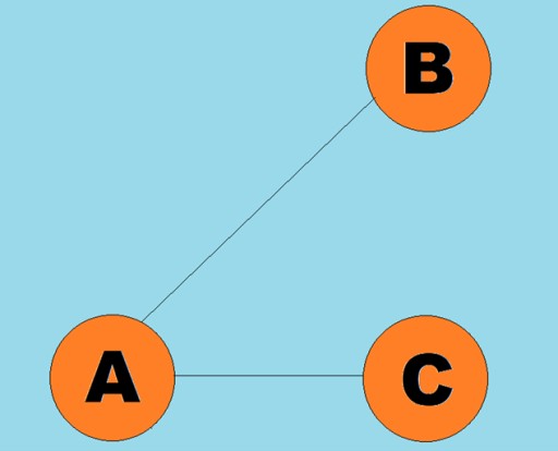
Garis penghubung tidak berarah dipanggil tepi: Garis berarah dipanggil lengkok: 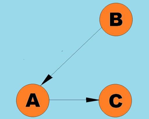Biasanya, graf diwakili oleh gambar rajah di mana beberapa bucu disambungkan oleh tepi (arka). Graf yang tepinya menunjukkan arah lintasan dipanggil graf terarah. Jika graf disambungkan dengan tepi yang tidak menunjukkan arah traversal, maka kita katakan ia adalah graf tidak berarah. Ini bermakna pergerakan boleh dilakukan dalam kedua-dua arah: kedua-dua dari bucu A ke bucu B, dan dari bucu B ke bucu A. Graf bersambung ialah graf di mana sekurang-kurangnya satu laluan menuju dari setiap bucu ke mana-mana bucu lain (seperti dalam contoh di atas). 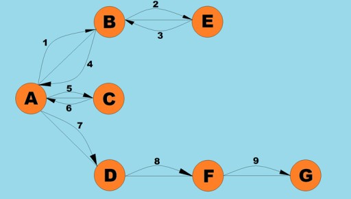Jika ini tidak berlaku, maka graf dikatakan terputus sambungan: 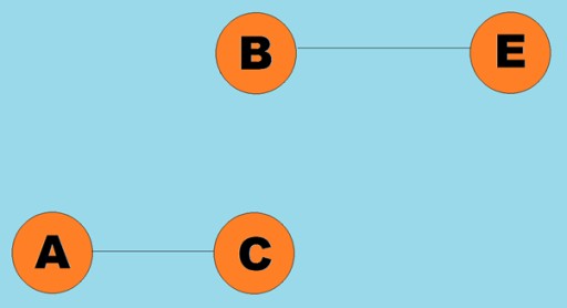Pemberat juga boleh ditetapkan pada tepi (arka). Pemberat ialah nombor yang mewakili, contohnya, jarak fizikal antara dua bucu (atau masa perjalanan relatif antara dua bucu). Graf ini dipanggil graf berwajaran:

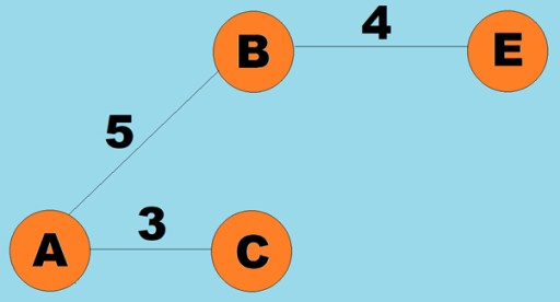
3. Algoritma pencarian laluan (depth-first, breadth-first)

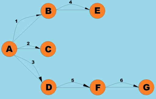
Salah satu operasi asas yang dilakukan dengan graf ialah menentukan semua bucu yang boleh dicapai dari bucu tertentu. Bayangkan anda cuba menentukan cara anda boleh menaiki bas dari satu bandar ke bandar lain, termasuk kemungkinan pemindahan. Sesetengah bandar boleh dicapai secara terus, manakala sesetengahnya hanya boleh dicapai dengan melalui bandar lain. Terdapat banyak situasi lain di mana anda mungkin perlu mencari semua bucu yang boleh anda capai dari bucu tertentu. Terdapat dua cara utama untuk melintasi graf: kedalaman-didahulukan dan keluasan-didahulukan. Kami akan meneroka kedua-duanya. Kedua-dua kaedah merentasi semua bucu yang bersambung. Untuk meneroka lebih lanjut algoritma depth-first dan breadth-first, kami akan menggunakan graf berikut: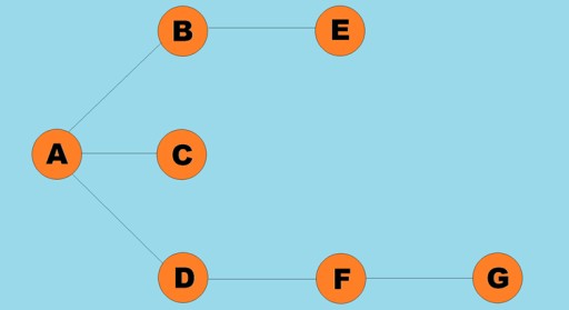

Carian mendalam-pertama

Ini adalah salah satu kaedah traversal graf yang paling biasa. Strategi kedalaman pertama ialah pergi sedalam mungkin dalam graf. Kemudian selepas mencapai jalan buntu, kita kembali ke puncak terdekat yang sebelum ini tidak pernah dikunjungi bucu bersebelahan. Algoritma ini menyimpan maklumat pada timbunan tentang tempat untuk kembali apabila jalan buntu dicapai. Peraturan untuk carian mendalam dahulu:

1. Lawati bucu bersebelahan yang tidak dilawati sebelum ini, tandai sebagai dilawati dan tolaknya ke atas timbunan.
2. Beralih ke puncak ini.
3. Ulang langkah 1.
4. Jika langkah 1 adalah mustahil, kembali ke bucu sebelumnya dan cuba lakukan langkah 1. Jika itu tidak mungkin, kemudian kembali ke bucu sebelum yang itu, dan seterusnya, sehingga kita menemui bucu dari mana kita boleh meneruskan traversal.
5. Teruskan sehingga semua bucu berada pada timbunan.

Mari kita lihat rupa kod Java untuk algoritma ini:

public class Graph {
  private final int MAX_VERTS = 10;
  private Vertex vertexArray[]; // Array of vertices
  private int adjMat[][]; // Adjacency matrix
  private int nVerts; // Current number of vertices
  private Stack stack;

  public Graph() { // Initialize internal fields
     vertexArray = new Vertex[MAX_VERTS];
     adjMat = new int[MAX_VERTS][MAX_VERTS];
     nVerts = 0;
     for (int j = 0; j < MAX_VERTS; j++) {
        for (int k = 0; k < MAX_VERTS; k++) {
           adjMat[j][k] = 0;
        }
     }
     stack = new Stack<>();
  }

  public void addVertex(char lab) {
     vertexArray[nVerts++] = new Vertex(lab);
  }

  public void addEdge(int start, int end) {
     adjMat[start][end] = 1;
     adjMat[end][start] = 1;
  }

  public void displayVertex(int v) {
     System.out.println(vertexArray[v].getLabel());
  }

  public void dfs() { // Depth-first search
     vertexArray[0].setVisited(true); // Take the first vertex
     displayVertex(0);
     stack.push(0);

     while (!stack.empty()) {
        int v = getAdjUnvisitedVertex(stack.peek()); // Return the index of the adjacent vertex: if any, 1; if not, -1
        if (v == -1) { // If there is no unvisited adjacent vertex
           stack.pop(); // The element is removed from the stack
        }
        else {
           vertexArray[v].setVisited(true);
           displayVertex(v);
           stack.push(v); // The element goes on top of the stack
        }
     }

     for (int j = 0; j < nVerts; j++) {  // Reset the flags
        vertexArray[j].visited = false;
     }

  }

  private int getAdjUnvisitedVertex(int v) {
     for (int j = 0; j < nVerts; j++) {
        if (adjMat[v][j] == 1 && vertexArray[j].visited == false) {
           return j; // Returns the first vertex found
        }
     }
     return -1;
  }
}

Puncak kelihatan seperti ini:

public class Vertex {
  private char label;  // for example, 'A'
  public boolean visited;

  public Vertex(final char label) {
     this.label = label;
     visited = false;
  }

  public char getLabel() {
     return this.label;
  }

  public boolean isVisited() {
     return this.visited;
  }

  public void setVisited(final boolean visited) {
     this.visited = visited;
  }
}

Mari jalankan algoritma ini dengan bucu tertentu dan lihat sama ada ia berfungsi dengan betul:

public class Solution {
  public static void main(String[] args) {
     Graph graph = new Graph();
     graph.addVertex('A'); //0
     graph.addVertex('B'); //1
     graph.addVertex('C'); //2
     graph.addVertex('D'); //3
     graph.addVertex('E'); //4
     graph.addVertex('F'); //5
     graph.addVertex('G'); //6

     graph.addEdge(0,1);
     graph.addEdge(0,2);
     graph.addEdge(0,3);
     graph.addEdge(1,4);
     graph.addEdge(3,5);
     graph.addEdge(5,6);

     System.out.println("Visits: ");
     graph.dfs();
  }
}

Output konsol: Memandangkan kita mempunyai matriks bersebelahan dan menggunakan gelung dalam gelung, kerumitan masa ialah O(N²).

Keluasan-pertama carian

Seperti carian mendalam-pertama, algoritma ini adalah salah satu kaedah traversal graf yang paling mudah dan paling asas. Intinya ialah kita mempunyai beberapa puncak semasa. Kami meletakkan semua bucu bersebelahan yang tidak dilawati ke dalam baris gilir dan pilih elemen seterusnya (iaitu bucu yang disimpan di kepala baris gilir), yang menjadi bucu semasa... Memecahkan algoritma ini kepada berperingkat, kita boleh mengenal pasti langkah berikut:

1. Lawati puncak seterusnya yang belum dilawati sebelum ini bersebelahan dengan puncak semasa, tandai sebagai dilawati lebih awal dan tambahkannya pada baris gilir.
2. Jika langkah #1 tidak dapat dilakukan, kemudian keluarkan bucu daripada baris gilir dan jadikannya bucu semasa.
3. Jika langkah #1 dan #2 tidak dapat dilakukan, maka kita telah selesai melintasi — setiap bucu telah dilalui (jika kita mempunyai graf bersambung).

Kelas graf di sini hampir sama dengan yang kami gunakan untuk algoritma carian pertama mendalam, kecuali kaedah carian itu sendiri dan fakta bahawa baris gilir menggantikan tindanan dalaman:

public class Graph {
  private final int MAX_VERTS = 10;
  private Vertex vertexList[]; // Array of vertices
  private int adjMat[][]; // Adjacency matrix
  private int nVerts; // Current number of vertices
  private Queue queue;

  public Graph() {
     vertexList = new Vertex[MAX_VERTS];
     adjMat = new int[MAX_VERTS][MAX_VERTS];
     nVerts = 0;
     for (int j = 0; j < MAX_VERTS; j++) {
        for (int k = 0; k < MAX_VERTS; k++) {  // Fill the adjacency matrix with zeros
           adjMat[j][k] = 0;
        }
     }
     queue = new PriorityQueue<>();
  }

  public void addVertex(char lab) {
     vertexList[nVerts++] = new Vertex(lab);
  }

  public void addEdge(int start, int end) {
     adjMat[start][end] = 1;
     adjMat[end][start] = 1;
  }

  public void displayVertex(int v) {
     System.out.println(vertexList[v].getLabel());
  }

  public void bfc() { // Depth-first search
     vertexList[0].setVisited(true);
     displayVertex(0);
     queue.add(0);
     int v2;

     while (!queue.isEmpty()) {
        int v = queue.remove();

        while((v2 = getAdjUnvisitedVertex(v))!=-1) {// The loop runs until every adjacent vertex is found and added to the queue
           vertexList[v2].visited = true;
           displayVertex(v2);
           queue.add(v2);
        }
     }

     for (int j = 0; j < nVerts; j++) {  // Reset the flags
        vertexList[j].visited = false;
     }

  }

  private int getAdjUnvisitedVertex(int v) {
     for (int j = 0; j < nVerts; j++) {
        if (adjMat[v][j] == 1 && vertexList[j].visited == false) {
           return j; // Returns the first vertext found
        }
     }
     return -1;
  }
}

Kelas Vertex adalah sama dengan yang kami gunakan dengan algoritma carian mendalam-pertama. Mari kita lakukan algoritma ini:

public class Solution {
  public static void main(String[] args) {
     Graph graph = new Graph();
     graph.addVertex('A'); //0
     graph.addVertex('B'); //1
     graph.addVertex('C'); //2
     graph.addVertex('D'); //3
     graph.addVertex('E'); //4
     graph.addVertex('F'); //5
     graph.addVertex('G'); //6

     graph.addEdge(0,1);
     graph.addEdge(0,2);
     graph.addEdge(0,3);
     graph.addEdge(1,4);
     graph.addEdge(3,5);
     graph.addEdge(5,6);

     System.out.println("Visits: ");
     graph.bfc();
  }
}

Output konsol: Sekali lagi: kami mempunyai matriks bersebelahan dan menggunakan gelung bersarang dalam gelung, jadi kerumitan masa algoritma di atas ialah O(N²).

4. Algoritma Dijkstra

Seperti yang dinyatakan sebelum ini, graf boleh diarahkan atau tidak terarah. Dan anda akan ingat bahawa mereka juga boleh ditimbang. Perhubungan model graf berwajaran dan terarah yang sering ditemui dalam kehidupan sebenar: contohnya, peta bandar di mana bandar adalah bucu, dan tepi di antaranya ialah jalan raya dengan trafik sehala, mengalir ke arah tepi yang diarahkan. Katakan anda sebuah syarikat pengangkutan dan anda perlu mencari laluan terpendek antara dua bandar yang jauh. Bagaimana anda akan melakukannya? Mencari laluan terpendek antara dua bucu adalah salah satu masalah yang paling biasa diselesaikan menggunakan graf berwajaran. Untuk menyelesaikan masalah ini, kami menggunakan algoritma Dijkstra. Sebaik sahaja anda menjalankannya, anda akan mengetahui laluan terpendek dari puncak awal yang diberikan kepada setiap satu yang lain. Apakah langkah-langkah algoritma ini? Saya akan cuba menjawab soalan ini. Langkah-langkah algoritma Dijkstra:

• Langkah 1: Cari nod bersebelahan yang mempunyai kos terendah untuk menavigasi ke (berat tepi terendah). Anda berdiri di awal-awal lagi dan memikirkan ke mana hendak pergi: ke nod A atau nod B. Berapakah kos untuk berpindah ke setiap nod ini?
• Langkah 2: hitung jarak perjalanan ke semua jiran nod В yang masih belum dilawati oleh algoritma semasa melintasi tepi dari В. Jika jarak baharu kurang daripada jarak lama, maka laluan melalui tepi B menjadi laluan terpendek baharu untuk bucu ini.
• Langkah 3: tandakan bucu B sebagai dilawati.
• Langkah 4: Pergi ke langkah 1.

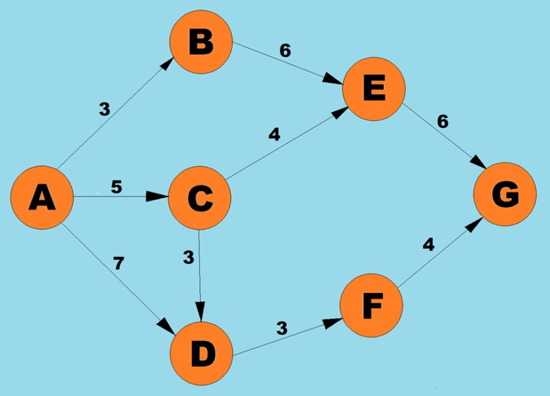Kami akan mengulangi langkah ini dalam satu gelung sehingga semua bucu telah dilawati. Mari kita pertimbangkan graf berwajaran berikut: Menggunakan algoritma di atas, kita akan menentukan laluan terpendek dari A ke G:

1. Terdapat tiga laluan yang mungkin untuk puncak A: ke B dengan berat 3, ke С dengan berat 5, dan ke D dengan berat 7. Menurut langkah pertama algoritma, kami memilih nod dengan kos terendah (berat tepi). Dalam kes ini, B.

2. Memandangkan satu-satunya jiran B yang tidak dilawati ialah bucu Е, kami menyemak laluan yang akan berlaku jika kami melalui bucu ini. 3(AB) + 6(BE) = 9.

   Oleh itu, kami merekodkan bahawa laluan terpendek semasa dari A ke E ialah 9.

3. Memandangkan kerja kami dengan bucu B selesai, kami meneruskan untuk memilih bucu seterusnya yang tepinya mempunyai berat minimum.

   Daripada bucu A dan B, kemungkinannya ialah bucu D (7), C (5), atau E (6).

   Tepi ke С mempunyai berat terkecil, jadi kita pergi ke puncak ini.

4. Seterusnya, seperti sebelum ini, kita dapati laluan terpendek ke bucu jiran apabila melalui C:

   • AD = 5 (AC) + 3 (CD) = 8, tetapi memandangkan laluan terpendek sebelumnya (AC = 7) adalah kurang daripada laluan ini melalui С, kami mengekalkan laluan terpendek (AC = 7) tidak berubah.

   • CE = 5(AC) + 4(CE) = 9. Laluan terpendek baharu ini adalah sama dengan laluan sebelumnya, jadi kami juga membiarkannya tidak berubah.

5. Daripada bucu boleh diakses terdekat (E dan D), pilih bucu dengan berat tepi terkecil, iaitu D (3).

6. Kami mencari jalan terpendek ke jirannya F.

   AF = 7(AD) + 3(DF) = 9

7. Daripada bucu boleh diakses terdekat (E dan F), pilih bucu dengan berat tepi terkecil, iaitu F (3).

8. Cari jalan terpendek ke jirannya G.

   AG = 7(AD) + 3(DF) + 4(FG) = 14

   Jadi, kami telah menemui laluan dari A ke G.

   Tetapi untuk memastikan ia adalah yang terpendek, kita juga mesti melakukan langkah kita pada puncak E.

9. Oleh kerana bucu G tidak mempunyai bucu jiran yang ditunjuk oleh tepi terarah, kita hanya tinggal bucu E, jadi kita memilihnya.

10. Cari jalan terpendek ke jiran G.

    AG = 3 (AB) + 6 (BE) + 6 (EG) = 15. Laluan ini lebih panjang daripada laluan terpendek sebelumnya (AG (14)), jadi kita biarkan laluan ini tidak berubah.

    Memandangkan tiada bucu menuju dari G, tidak masuk akal untuk menjalankan langkah pada algoritma pada bucu ini. Ini bermakna bahawa kerja algoritma telah selesai.

Seperti yang saya katakan sebelum ini, selain daripada mencari laluan terpendek untuk AG, kami juga memperoleh laluan terpendek dari bucu A ke setiap bucu lain (AB, AC, AD, AE, AF). Nah, kini tiba masanya untuk melihat bagaimana ini boleh dilakukan di Jawa. Mari kita mulakan dengan kelas puncak:

public class Vertex {
   private char label;
   private boolean isInTree;

   public Vertex(char label) {
       this.label = label;
       this.isInTree = false;
   }

   public char getLabel() {
       return label;
   }

   public void setLabel(char label) {
       this.label = label;
   }

   public boolean isInTree() {
       return isInTree;
   }

   public void setInTree(boolean inTree) {
       isInTree = inTree;
   }
}

Kelas bucu hampir sama dengan kelas bucu yang digunakan untuk carian pertama keluasan. Untuk memaparkan laluan terpendek, kami memerlukan kelas baharu yang akan mengandungi data yang kami perlukan:

public class Path { // A class that contains the distance and the previous and traversed vertices
   private int distance; // Current distance from the starting vertex
   private List parentVertices; // Current parent vertex

   public Path(int distance) {
       this.distance = distance;
       this.parentVertices = new ArrayList<>();
   }

   public int getDistance() {
       return distance;
   }

   public void setDistance(int distance) {
       this.distance = distance;
   }

   public List getParentVertices() {
       return parentVertices;
   }

   public void setParentVertices(List parentVertices) {
       this.parentVertices = parentVertices;
   }
}

Dalam kelas ini, kita boleh melihat jumlah jarak laluan dan bucu yang akan dilalui apabila melalui laluan terpendek. Dan sekarang mari kita lihat kelas di mana kita sebenarnya melintasi laluan terpendek melalui graf. Jadi di sini kita mempunyai kelas Graf:

public class Graph {
   private final int MAX_VERTS = 10;// Maximum number of vertices
   private final int INFINITY = 100000000; // This number represents infinity
   private Vertex vertexList[]; // List of vertices
   private int relationMatrix[][]; // Matrix of edges between vertices
   private int numberOfVertices; // Current number of vertices
   private int numberOfVerticesInTree; // Number of visited vertices in the tree
   private List shortestPaths; // List of shortest paths
   private int currentVertex; // Current vertex
   private int startToCurrent; // Distance to currentVertex

   public Graph() {
       vertexList = new Vertex[MAX_VERTS]; // Adjacency matrix
       relationMatrix = new int[MAX_VERTS][MAX_VERTS];
       numberOfVertices = 0;
       numberOfVerticesInTree = 0;
       for (int i = 0; i < MAX_VERTS; i++) { // Fill the adjacency matrix
           for (int k = 0; k < MAX_VERTS; k++) { // with "infinity"
               relationMatrix[i][k] = INFINITY; // Assign default values
               shortestPaths = new ArrayList<>(); // Assign an empty list
           }
       }
   }

   public void addVertex(char lab) {// Assign new vertices
       vertexList[numberOfVertices++] = new Vertex(lab);
   }

   public void addEdge(int start, int end, int weight) {
       relationMatrix[start][end] = weight; // Set weighted edges between vertices
   }

   public void path() { // Choose the shortest path
       // Set the initial vertex data
       int startTree = 0; // Start from vertex 0
       vertexList[startTree].setInTree(true); // Include the first element in the tree
       numberOfVerticesInTree = 1;

       // Fill out the shortest paths for vertices adjacent to the initial vertex
       for (int i = 0; i < numberOfVertices; i++) {
           int tempDist = relationMatrix[startTree][i];
           Path path = new Path(tempDist);
           path.getParentVertices().add(0);// The starting vertex will always be a parent vertex
           shortestPaths.add(path);
       }
       // Until every vertex is in the tree
       while (numberOfVerticesInTree < numberOfVertices) { // Do this until the number of of vertices in the tree equals the total number of vertices
           int indexMin = getMin();// Get the index of the of the vertex with the smallest distance from the vertices not yet in the tree
           int minDist = shortestPaths.get(indexMin).getDistance(); // Minimum distance to the vertices not yet in the tree

           if (minDist == INFINITY) {
               System.out.println("The graph has an unreachable vertex");
               break; // If only unreachable vertices have not been visited, then we exit the loop
           } else {
               currentVertex = indexMin; // Set currentVert to the index of the current vertex
               startToCurrent = shortestPaths.get(indexMin).getDistance(); // Set the distance to the current vertex
           }

           vertexList[currentVertex].setInTree(true);  // Add the current vertex to the tree
           numberOfVerticesInTree++; // Increase the count of vertices in the tree
           updateShortestPaths(); // Update the list of shortest paths
       }

       displayPaths(); // Display the results on the console
   }

   public void clear() { // Clear the tree
       numberOfVerticesInTree = 0;
       for (int i = 0; i < numberOfVertices; i++) {
           vertexList[i].setInTree(false);
       }
   }

   private int getMin() {
       int minDist = INFINITY; // The distance of the initial shortest path is taken to be infinite
       int indexMin = 0;
       for (int i = 1; i < numberOfVertices; i++) { // For each vertex
           if (!vertexList[i].isInTree() && shortestPaths.get(i).getDistance() < minDist) { // If the vertex is not yet in the tree and the distance to the vertex is less than the current minimum
               minDist = shortestPaths.get(i).getDistance(); // then update the minimum
               indexMin = i; // Update the index of the vertex with the minimum distance
           }
       }
       return indexMin; // Returns the index of the vertex with the smallest distance among those not yet in the tree
   }

   private void updateShortestPaths() {
       int vertexIndex = 1; // The initial vertex is skipped
       while (vertexIndex < numberOfVertices) { // Run over the columns

           if (vertexList[vertexIndex].isInTree()) { // If the column vertex is already in the tree, then we skip it
               vertexIndex++;
               continue;
           }
           // Calculate the distance for one element sPath
           // Get the edge from currentVert to column
           int currentToFringe = relationMatrix[currentVertex][vertexIndex];
           // Add up all the distances
           int startToFringe = startToCurrent + currentToFringe;
           // Determine the distance to the current vertexIndex
           int shortPathDistance = shortestPaths.get(vertexIndex).getDistance();

           // Compare the distance through currentVertex with the current distance in the vertex with index vertexIndex
           if (startToFringe < shortPathDistance) { // If it is smaller, then the vertex at vertexIndex is assigned the new shortest path
               List newParents = new ArrayList<>(shortestPaths.get(currentVertex).getParentVertices()); // Create a copy of the list of vertices of vertex currentVert's parents
               newParents.add(currentVertex); // And add currentVertex to it as the previous vertex
               shortestPaths.get(vertexIndex).setParentVertices(newParents); // Save the new path
               shortestPaths.get(vertexIndex).setDistance(startToFringe); // Save the new distance
           }
           vertexIndex++;
       }
   }

   private void displayPaths() { // A method for displaying the shortest paths on the screen
       for (int i = 0; i < numberOfVertices; i++) {
           System.out.print(vertexList[i].getLabel() + " = ");
           if (shortestPaths.get(i).getDistance() == INFINITY) {
               System.out.println("0");
           } else {
               String result = shortestPaths.get(i).getDistance() + " (";
               List parents = shortestPaths.get(i).getParentVertices();
               for (int j = 0; j < parents.size(); j++) {
                   result += vertexList[parents.get(j)].getLabel() + " -> ";
               }
               System.out.println(result + vertexList[i].getLabel() + ")");
           }
       }
   }
}

Jadi itu semua keajaiban =) Sekarang, mari kita lihat algoritma ini dalam tindakan:

public class Solution {

   public static void main(String[] args) {
       Graph graph = new Graph();
       graph.addVertex('A');
       graph.addVertex('B');
       graph.addVertex('C');
       graph.addVertex('D');
       graph.addVertex('E');
       graph.addVertex('F');
       graph.addVertex('G');

       graph.addEdge(0, 1, 3);
       graph.addEdge(0, 2, 5);
       graph.addEdge(0, 3, 7);
       graph.addEdge(1, 4, 6);
       graph.addEdge(2, 4, 4);
       graph.addEdge(2, 3, 3);
       graph.addEdge(3, 5, 3);
       graph.addEdge(4, 6, 6);
       graph.addEdge(5, 6, 4);

       System.out.println("The following nodes form the shortest paths from node A:");
       graph.path();
       graph.clear();
   }
}

Dan output konsol adalah ini: Kerumitan masa algoritma ini tidak lain adalah O(N²), kerana kami mempunyai gelung bersarang. Itu sahaja yang saya dapat hari ini. Terima kasih atas perhatian anda!