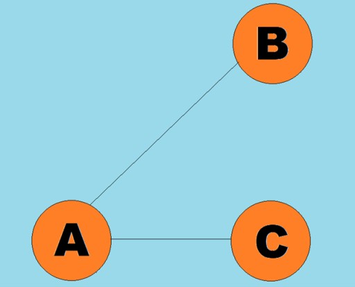
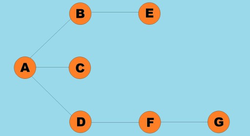
无向连接线称为边: 有向线称为弧:通常,图由其中一些顶点通过边(弧)连接的图来表示。边指示遍历方向的图称为有向图。如果一个图是由不指示遍历方向的边连接的,那么我们说它是无向图。这意味着可以在两个方向上移动:从顶点 A 到顶点 B,以及从顶点 B 到顶点 A。连通图是其中至少一条路径从每个顶点通向任何其他顶点的图(如上面的例子)。如果不是这种情况,则该图被称为断开连接:权重也可以分配给边(弧)。权重是表示例如两个顶点之间的物理距离(或两个顶点之间的相对行进时间)的数字。这些图称为加权图:
publicclassGraph{privatefinalint MAX_VERTS =10;privateVertex vertexArray[];// Array of verticesprivateint adjMat[][];// Adjacency matrixprivateint nVerts;// Current number of verticesprivateStack stack;publicGraph(){// Initialize internal fields
vertexArray =newVertex[MAX_VERTS];
adjMat =newint[MAX_VERTS][MAX_VERTS];
nVerts =0;for(int j =0; j < MAX_VERTS; j++){for(int k =0; k < MAX_VERTS; k++){
adjMat[j][k]=0;}}
stack =newStack<>();}publicvoidaddVertex(char lab){
vertexArray[nVerts++]=newVertex(lab);}publicvoidaddEdge(int start,int end){
adjMat[start][end]=1;
adjMat[end][start]=1;}publicvoiddisplayVertex(int v){System.out.println(vertexArray[v].getLabel());}publicvoiddfs(){// Depth-first search
vertexArray[0].setVisited(true);// Take the first vertexdisplayVertex(0);
stack.push(0);while(!stack.empty()){int v =getAdjUnvisitedVertex(stack.peek());// Return the index of the adjacent vertex: if any, 1; if not, -1if(v ==-1){// If there is no unvisited adjacent vertex
stack.pop();// The element is removed from the stack}else{
vertexArray[v].setVisited(true);displayVertex(v);
stack.push(v);// The element goes on top of the stack}}for(int j =0; j < nVerts; j++){// Reset the flags
vertexArray[j].visited =false;}}privateintgetAdjUnvisitedVertex(int v){for(int j =0; j < nVerts; j++){if(adjMat[v][j]==1&& vertexArray[j].visited ==false){return j;// Returns the first vertex found}}return-1;}}
顶点看起来像这样:
publicclassVertex{privatechar label;// for example, 'A'publicboolean visited;publicVertex(finalchar label){this.label = label;
visited =false;}publicchargetLabel(){returnthis.label;}publicbooleanisVisited(){returnthis.visited;}publicvoidsetVisited(finalboolean visited){this.visited = visited;}}
publicclassGraph{privatefinalint MAX_VERTS =10;privateVertex vertexList[];// Array of verticesprivateint adjMat[][];// Adjacency matrixprivateint nVerts;// Current number of verticesprivateQueue queue;publicGraph(){
vertexList =newVertex[MAX_VERTS];
adjMat =newint[MAX_VERTS][MAX_VERTS];
nVerts =0;for(int j =0; j < MAX_VERTS; j++){for(int k =0; k < MAX_VERTS; k++){// Fill the adjacency matrix with zeros
adjMat[j][k]=0;}}
queue =newPriorityQueue<>();}publicvoidaddVertex(char lab){
vertexList[nVerts++]=newVertex(lab);}publicvoidaddEdge(int start,int end){
adjMat[start][end]=1;
adjMat[end][start]=1;}publicvoiddisplayVertex(int v){System.out.println(vertexList[v].getLabel());}publicvoidbfc(){// Depth-first search
vertexList[0].setVisited(true);displayVertex(0);
queue.add(0);int v2;while(!queue.isEmpty()){int v = queue.remove();while((v2 =getAdjUnvisitedVertex(v))!=-1){// The loop runs until every adjacent vertex is found and added to the queue
vertexList[v2].visited =true;displayVertex(v2);
queue.add(v2);}}for(int j =0; j < nVerts; j++){// Reset the flags
vertexList[j].visited =false;}}privateintgetAdjUnvisitedVertex(int v){for(int j =0; j < nVerts; j++){if(adjMat[v][j]==1&& vertexList[j].visited ==false){return j;// Returns the first vertext found}}return-1;}}
publicclassPath{// A class that contains the distance and the previous and traversed verticesprivateint distance;// Current distance from the starting vertexprivateList parentVertices;// Current parent vertexpublicPath(int distance){this.distance = distance;this.parentVertices =newArrayList<>();}publicintgetDistance(){return distance;}publicvoidsetDistance(int distance){this.distance = distance;}publicListgetParentVertices(){return parentVertices;}publicvoidsetParentVertices(List parentVertices){this.parentVertices = parentVertices;}}
publicclassGraph{privatefinalint MAX_VERTS =10;// Maximum number of verticesprivatefinalint INFINITY =100000000;// This number represents infinityprivateVertex vertexList[];// List of verticesprivateint relationMatrix[][];// Matrix of edges between verticesprivateint numberOfVertices;// Current number of verticesprivateint numberOfVerticesInTree;// Number of visited vertices in the treeprivateList shortestPaths;// List of shortest pathsprivateint currentVertex;// Current vertexprivateint startToCurrent;// Distance to currentVertexpublicGraph(){
vertexList =newVertex[MAX_VERTS];// Adjacency matrix
relationMatrix =newint[MAX_VERTS][MAX_VERTS];
numberOfVertices =0;
numberOfVerticesInTree =0;for(int i =0; i < MAX_VERTS; i++){// Fill the adjacency matrixfor(int k =0; k < MAX_VERTS; k++){// with "infinity"
relationMatrix[i][k]= INFINITY;// Assign default values
shortestPaths =newArrayList<>();// Assign an empty list}}}publicvoidaddVertex(char lab){// Assign new vertices
vertexList[numberOfVertices++]=newVertex(lab);}publicvoidaddEdge(int start,int end,int weight){
relationMatrix[start][end]= weight;// Set weighted edges between vertices}publicvoidpath(){// Choose the shortest path// Set the initial vertex dataint startTree =0;// Start from vertex 0
vertexList[startTree].setInTree(true);// Include the first element in the tree
numberOfVerticesInTree =1;// Fill out the shortest paths for vertices adjacent to the initial vertexfor(int i =0; i < numberOfVertices; i++){int tempDist = relationMatrix[startTree][i];Path path =newPath(tempDist);
path.getParentVertices().add(0);// The starting vertex will always be a parent vertex
shortestPaths.add(path);}// Until every vertex is in the treewhile(numberOfVerticesInTree < numberOfVertices){// Do this until the number of of vertices in the tree equals the total number of verticesint indexMin =getMin();// Get the index of the of the vertex with the smallest distance from the vertices not yet in the treeint minDist = shortestPaths.get(indexMin).getDistance();// Minimum distance to the vertices not yet in the treeif(minDist == INFINITY){System.out.println("The graph has an unreachable vertex");break;// If only unreachable vertices have not been visited, then we exit the loop}else{
currentVertex = indexMin;// Set currentVert to the index of the current vertex
startToCurrent = shortestPaths.get(indexMin).getDistance();// Set the distance to the current vertex}
vertexList[currentVertex].setInTree(true);// Add the current vertex to the tree
numberOfVerticesInTree++;// Increase the count of vertices in the treeupdateShortestPaths();// Update the list of shortest paths}displayPaths();// Display the results on the console}publicvoidclear(){// Clear the tree
numberOfVerticesInTree =0;for(int i =0; i < numberOfVertices; i++){
vertexList[i].setInTree(false);}}privateintgetMin(){int minDist = INFINITY;// The distance of the initial shortest path is taken to be infiniteint indexMin =0;for(int i =1; i < numberOfVertices; i++){// For each vertexif(!vertexList[i].isInTree()&& shortestPaths.get(i).getDistance()< minDist){// If the vertex is not yet in the tree and the distance to the vertex is less than the current minimum
minDist = shortestPaths.get(i).getDistance();// then update the minimum
indexMin = i;// Update the index of the vertex with the minimum distance}}return indexMin;// Returns the index of the vertex with the smallest distance among those not yet in the tree}privatevoidupdateShortestPaths(){int vertexIndex =1;// The initial vertex is skippedwhile(vertexIndex < numberOfVertices){// Run over the columnsif(vertexList[vertexIndex].isInTree()){// If the column vertex is already in the tree, then we skip it
vertexIndex++;continue;}// Calculate the distance for one element sPath// Get the edge from currentVert to columnint currentToFringe = relationMatrix[currentVertex][vertexIndex];// Add up all the distancesint startToFringe = startToCurrent + currentToFringe;// Determine the distance to the current vertexIndexint shortPathDistance = shortestPaths.get(vertexIndex).getDistance();// Compare the distance through currentVertex with the current distance in the vertex with index vertexIndexif(startToFringe < shortPathDistance){// If it is smaller, then the vertex at vertexIndex is assigned the new shortest pathList newParents =newArrayList<>(shortestPaths.get(currentVertex).getParentVertices());// Create a copy of the list of vertices of vertex currentVert's parents
newParents.add(currentVertex);// And add currentVertex to it as the previous vertex
shortestPaths.get(vertexIndex).setParentVertices(newParents);// Save the new path
shortestPaths.get(vertexIndex).setDistance(startToFringe);// Save the new distance}
vertexIndex++;}}privatevoiddisplayPaths(){// A method for displaying the shortest paths on the screenfor(int i =0; i < numberOfVertices; i++){System.out.print(vertexList[i].getLabel()+" = ");if(shortestPaths.get(i).getDistance()== INFINITY){System.out.println("0");}else{String result = shortestPaths.get(i).getDistance()+" (";List parents = shortestPaths.get(i).getParentVertices();for(int j =0; j < parents.size(); j++){
result += vertexList[parents.get(j)].getLabel()+" -> ";}System.out.println(result + vertexList[i].getLabel()+")");}}}}
这就是神奇之处 =) 现在,让我们看看这个算法的实际应用:
publicclassSolution{publicstaticvoidmain(String[] args){Graph graph =newGraph();
graph.addVertex('A');
graph.addVertex('B');
graph.addVertex('C');
graph.addVertex('D');
graph.addVertex('E');
graph.addVertex('F');
graph.addVertex('G');
graph.addEdge(0,1,3);
graph.addEdge(0,2,5);
graph.addEdge(0,3,7);
graph.addEdge(1,4,6);
graph.addEdge(2,4,4);
graph.addEdge(2,3,3);
graph.addEdge(3,5,3);
graph.addEdge(4,6,6);
graph.addEdge(5,6,4);System.out.println("The following nodes form the shortest paths from node A:");
graph.path();
graph.clear();}}
控制台输出是这样的:
以下节点形成从节点 A 开始的最短路径: A = 0 B = 3 (A -> B) C = 5 (A -> C) D = 7 (A -> D) E = 9 (A -> B - > E) F = 10 (A -> D -> F) G = 14 (A -> D -> F -> G)
 今天我们将讨论图以及与之相关的算法。图是编程中最灵活、最通用的结构之一。图G通常由一对集合来定义,即G = (V, R),其中:
 向线称为弧:
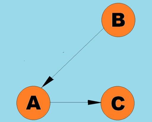 通常,图由其中一些顶点通过边(弧)连接的图来表示。边指示遍历方向的图称为有向图。如果一个图是由不指示遍历方向的边连接的,那么我们说它是无向图。这意味着可以在两个方向上移动:从顶点 A 到顶点 B,以及从顶点 B 到顶点 A。连通图是其中至少一条路径从每个顶点通向任何其他顶点的图(如上面的例子)。如果不是这种情况,则该图被称为断开连接:
 权重也可以分配给边(弧)。权重是表示例如两个顶点之间的物理距离(或两个顶点之间的相对行进时间)的数字。这些图称为加权图:
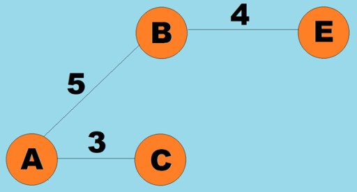
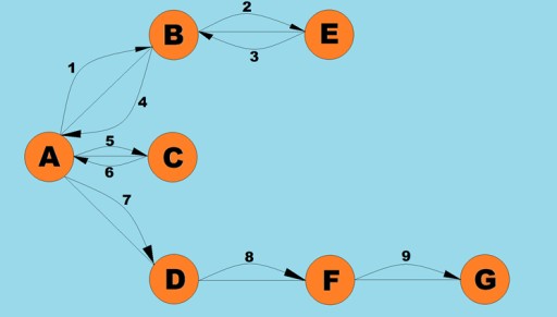 让我们看一下该算法的 Java 代码可能是什么样子:

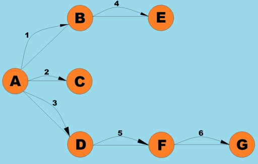 这里的图类与我们用于深度优先搜索算法的图类几乎相同,除了搜索方法本身以及队列取代了内部堆栈这一事实:
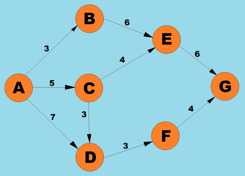 使用上述算法,我们将确定从 A 到 G 的最短路径:


GO TO FULL VERSION